from datasets import load_dataset

fashion_mnist = load_dataset("fashion_mnist")Stable Diffusion
In the previous chapter, we introduced diffusion models and the underlying idea of iterative refinement. By the end of the chapter, we could generate images, but training the model was time-consuming and we had no control over the images that were generated. In this chapter, we’ll see how to go from this to text-conditioned models that can efficiently generate images based on text descriptions, with a model called Stable Diffusion (SD) as a case study. Before we get to SD, though, we’ll first look at how conditional models work and go over some of the innovations that lead up to the text-to-image models we have today
Adding Control: Conditional Diffusion Models
Before we deal with the problem of generating images from text descriptions (a very challenging task!), let’s focus on something slightly easier first. We’ll see how we can steer our models outputs towards specific types or classes of images. We can use a method called conditioning, where the idea is to ask the model to generate not just any image, but an image belonging to a pre-defined class.
Model conditioning is a simple but effective idea. We’ll start from the same diffusion model we used in Chapter 3, with just a couple of changes. First, we’ll use a new dataset called Fashion MNIST instead of butterflies so that we can identify categories easily. Then, crucially, we’ll run two inputs through the model. Instead of just showing it how real images look like, we’ll also tell it the class every image belongs to. We hope the model will learn to associate images and labels, so it gets an idea about the distinctive features of sweaters, boots and the like.
Note that we are not interested in solving a classification problem – we don’t want the model to tell us the class, given an input image –. We still want it to perform the same task as in Chapter 3, namely: please, generate plausible images that look like they came from this dataset. The only difference is that we are giving it additional information about those images. We’ll use the same loss function and training strategy, as it’s the same task as before.
Preparing the Data
We need a dataset with distinct groups of images. Datasets intended for computer vision classification tasks are ideal for this purpose. We could start with something like the ImageNet dataset, which contains millions of images across 1000 classes. However, training models on this dataset would take an extremely long time. When approaching a new problem, it’s often a good idea to start with a smaller dataset first, to make sure everything works as expected. This keeps the feedback loop short, so we can iterate quickly and make sure we’re on the right track.
For this example, we could choose MNIST as we did in Chapter 3. To make things just a little bit different, we’ll choose Fashion MNIST instead. Fashion MNIST, developed and open-sourced by Zalando, is a replacement for MNIST that shares some of the same characteristics: a compact size, black & white images, and 10 classes. The main difference is that instead of being digits, classes correspond to different types of clothing and the images contain more detail than simple handwritten digits.
Let’s look at some examples.
clothes = fashion_mnist["train"]["image"][:8]
classes = fashion_mnist["train"]["label"][:8]
show_images(clothes, titles=classes, figsize=(4,2.5))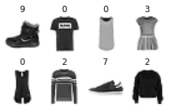
So class 0 means t-shirt, 2 is a sweater and 9 means boot. Here’s a list of the 10 categories in Fashion MNIST: https://www.kaggle.com/datasets/zalando-research/fashionmnist. We prepare our dataset and dataloader similarly to how we did it in Chapter 4, with the main difference that we’ll also include the class information as an input. Instead of resizing, in this case we’ll pad our image inputs (which have a size of 28 × 28 pixels) to 32 × 32, as we did in Chapter 3.
preprocess = transforms.Compose([
    transforms.RandomHorizontalFlip(),   # Randomly flip (data augmentation)
    transforms.ToTensor(),               # Convert to tensor (0, 1)
    transforms.Pad(2),                   # Add 2 pixels on all sides
    transforms.Normalize([0.5], [0.5]),  # Map to (-1, 1)
])
batch_size = 256
def transform(examples):
images = [preprocess(image.convert("L")) for image in examples["image"]]
return {"images": images, "labels": examples["label"]}
train_dataset = fashion_mnist["train"].with_transform(transform)
train_dataloader = torch.utils.data.DataLoader(
train_dataset, batch_size=batch_size, shuffle=True
)Creating a Class-Conditioned Model
If we use the UNet model from the diffusers library, we can provide our own custom conditioning information, because the code already supports it. Here we create a similar model to the one we used in Chapter 4, but we add a num_class_embeds argument to the UNet constructor. This argument tells the model that we’d like to use class labels as additional conditioning. We’ll use 10, because we have 10 classes in Fashion MNIST.
model = UNet2DModel(
    in_channels=1,   # 1 channel for grayscale images
    out_channels=1,  # output channels must also be 1
    sample_size=32,
    block_out_channels=(32, 64, 128, 256),
    norm_num_groups=8,
    num_class_embeds=10, # Enable class conditioning
)
To make predictions with this model, we must pass in the class labels as additional inputs to the forward method:
x = torch.randn((1, 1, 32, 32))
with torch.no_grad():
    out = model(x, timestep=7, class_labels=torch.tensor([2])).sample
out.shape
torch.Size([1, 1, 32, 32])
Note
You’ll notice we also pass something else to the model as conditioning: the timestep! That’s right, even the model from Chapter 4 can be considered a conditional diffusion model! We condition it on the timestep in the hopes that knowing how far we are in the diffusion process will help it generate more realistic images.
Internally, both the timestep and the class label are turned into embeddings that the model uses during its forward pass. At multiple stages throughout the UNet, these embeddings are projected onto a dimension that matches the number of channels in a given layer and are then added to the outputs of that layer. This means the conditioning information is fed to every block of the UNet, giving the model ample opportunity to learn how to use it effectively.
Training the Model
Adding noise works just as well on greyscale images as it did on the butterflies from Chapter 4.
# View a batch with different amounts of noise applied
scheduler = DDPMScheduler(num_train_timesteps=1000, beta_start=0.0001, beta_end=0.02)
timesteps = torch.linspace(0, 999, 8).long()
batch = next(iter(train_dataloader))
x = batch['images'][:8]
noise = torch.rand_like(x)
noised_x = scheduler.add_noise(x, noise, timesteps)
show_images((noised_x*0.5 + 0.5).clip(0, 1))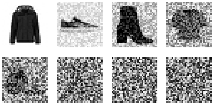
Our training loop is also almost exactly the same as in Chapter 4, except that we now pass the class labels for conditioning. Note that this is just additional information for the model, but it doesn’t affect our loss function in any way.
Note
We’ll also display some progress during training using the Python package tqdm. We can’t resist sharing this quote from their documentation (https://tqdm.github.io):
tqdmmeans “progress” in Arabic (taqadum, تقدّم) and is an abbreviation for “I love you so much” in Spanish (te quiero demasiado).
num_epochs = 25
lr = 3e-4
model = model.to(device) # The model we're training (defined in the previous section)
optimizer = torch.optim.AdamW(model.parameters(), lr=lr, eps=1e-5) # The optimizer
losses = [] # somewhere to store the loss values for later plotting

scheduler = DDPMScheduler(num_train_timesteps=1000, beta_start=0.0001, beta_end=0.02)

# Train the model (this takes a while!)
for epoch in (progress := tqdm(range(num_epochs))):
    for step, batch in (inner := tqdm(enumerate(train_dataloader), position=0, leave=True, total=len(train_dataloader))):
        # Load the input images
        clean_images = batch["images"].to(device)
        class_labels = batch["labels"].to(device)

        # Sample noise to add to the images
        noise = torch.randn(clean_images.shape).to(clean_images.device)

        # Sample a random timestep for each image
        timesteps = torch.randint(
            0,
            scheduler.num_train_timesteps,
            (clean_images.shape[0],),
            device=clean_images.device,
        ).long()

        # Add noise to the clean images according to the timestep
        noisy_images = scheduler.add_noise(clean_images, noise, timesteps)

        # Get the model prediction for the noise - note the use of class_labels
        noise_pred = model(noisy_images, timesteps, class_labels=class_labels, return_dict=False)[0]

        # Compare the prediction with the actual noise:
        loss = F.mse_loss(noise_pred, noise)

        # Display loss
        inner.set_postfix(loss=f"{loss.cpu().item():.3f}")

        # Store the loss for later plotting
        losses.append(loss.item())

        # Update the model parameters with the optimizer based on this loss
        loss.backward(loss)
        optimizer.step()
optimizer.zero_grad()plt.plot(losses);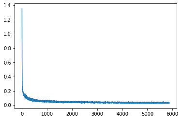
Sampling
Now we have a model that expects two inputs when making predictions: the image and the class label. We can create samples by beginning with random noise and then iteratively denoising, passing in whatever class label we’d like to generate:
def generate_from_class(class_to_generate, n_samples=8):
    sample = torch.randn(n_samples, 1, 32, 32).to(device)
    class_labels = [class_to_generate] * n_samples
    class_labels = torch.tensor(class_labels).to(device)

    for i, t in tqdm(enumerate(scheduler.timesteps)):
        # Get model pred
        with torch.no_grad():
            noise_pred = model(sample, t, class_labels=class_labels).sample

        # Update sample with step
        sample = scheduler.step(noise_pred, t, sample).prev_sample

    return sample.clip(-1, 1)*0.5 + 0.5
# Generate t-shirts (class 0)
images = generate_from_class(0)
show_images(images, nrows=2)1000it [00:21, 47.25it/s]
# Now generate some sneakers (class 7)
images = generate_from_class(7)
show_images(images, nrows=2)
1000it [00:21, 47.20it/s]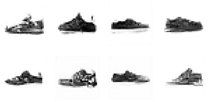
# ...or boots (class 9)
images = generate_from_class(9)
show_images(images, nrows=2)
1000it [00:21, 47.26it/s]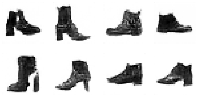
As you can see, the generated images are far from perfect. They’d probably get much better if we explored the architecture and trained for longer. But it’s amazing that the model not only learnt the shapes of different types of clothing, but also realized that shape 9 looks different than shape 0, just by sending this information alongside the training data. To put it in a slightly different way: the model is used to seeing the number 9 accompanying boots. When we ask it to generate an image and provide the 9, it responds with a boot.
Improving Efficiency: Latent Diffusion
Now that we can train a conditional model, all we need to do is scale it up and condition it on text instead of class labels, right? Well, not quite. As image size grows, so does the computational power required to work with those images. This is especially pronounced in an operation called self-attention, where the amount of operations grows quadratically with the number of inputs. A 128px square image has 4x as many pixels as a 64px square image, and so requires 16x (i.e. ) the memory and compute in a self-attention layer. This is a problem for anyone who’d like to generate high-resolution images!

Figure 2: The architecture introduced in Latent Diffusion Models TODO cite. Note the VAE encoder and decoder on the left for translating between pixel space and latent space
Latent diffusion tries to mitigate this issue by using a separate model called a Variational Auto-Encoder (VAE). As we saw in Chapter 3, VAEs can compress images to a smaller spatial dimension. The rationale behind this is that images tend to contain a large amount of redundant information - given enough training data, a VAE can hopefully learn to produce a much smaller representation of an input image and then reconstruct the image based on this small latent representation with a high degree of fidelity. The VAE used in SD takes in 3-channel images and produces a 4-channel latent representation with a reduction factor of 8 for each spatial dimension. That is, a 512px square input image will be compressed down to a 4x64x64 latent.
By applying the diffusion process on these smaller latent representations rather than on full-resolution images, we can get many of the benefits that would come from using smaller images (lower memory usage, fewer layers needed in the UNet, faster generation times…) and still decode the result back to a high-resolution image once we’re ready to view it. This innovation dramatically lowers the cost to train and run these models. The paper that introduced this idea (LDM TODO link by Rombach et al) demonstrated the power of this technique by training models conditioned on segmentation maps, class labels and text. The impressive results led to further collaboration between the authors and partners such as RunwayML, LAION, and EleutherAI to train a more powerful version of the model, which became Stable Diffusion.
Stable Diffusion: Components in Depth
Stable Diffusion is a text-conditioned latent diffusion model. Thanks to its popularity, there are hundreds of websites and apps that let you use it to create images with no technical knowledge required. It’s also very well-supported by libraries like diffusers, which let us sample an image with SD using a user-friendly pipeline:
pipe("Watercolor illustration of a rose").images[0]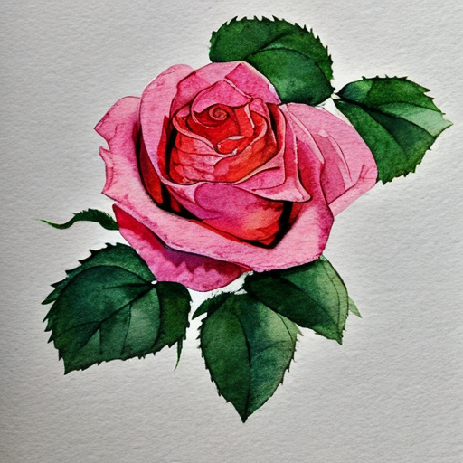
In this section we’ll explore all of the components that make this possible.
The Text Encoder
So how does Stable Diffusion understand text? Earlier on we showed how feeding additional information to the UNet allows us to have some additional control over the types of images generated. Given a noisy version of an image, the model is tasked with predicting the denoised version based on additional clues such as a class label. In the case of SD, the additional clue is the text prompt. At inference time, we can feed in the description of an image we’d like to see and some pure noise as a starting point, and the model does its best to denoise the random input into something that matches the caption.
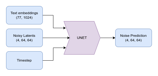
Figure 3: The text encoder turns an input string into text embeddings which are fed into the UNet along with the timestep and the noisy latents.
For this to work, we need to create a numeric representation of the text that captures relevant information about what it describes. To do this, SD leverages a pre-trained transformer model based on CLIP, which was also introduced in Chapter 2. The text encoder is a transformer model that takes in a sequence of tokens and produces a 1024-dimensional vector for each token (0r 768-dimensional in the case of SD version 1 which we’re using for the demonstrations in this section). Instead of combining these vectors into a single representation, we keep them separate and use them as conditioning for the UNet. This allows the UNet to make use of the information in each token separately, rather than just the overall meaning of the entire prompt. Because we’re extracting these text embeddings from the internal representation of the CLIP model, they are often called the “encoder hidden states”. Figure 3 shows the text encoder architecture.

Figure 5. Diagram showing the text encoding process which transforms the input prompt into a set of text embeddings (the encoder_hidden_states) which can then be fed in as conditioning to the UNet.
The first step to encode text is to follow a process called tokenization. This converts a sequence of characters into a sequence of numbers, where each number represents a group of various characters. Characters that are usually found together (like most common words) can be assigned a single token that represents the whole word or group. Long or complicated words, or words with many inflections, may be translated to multiple tokens, where each one usually represents a meaningful section of the word.
There is no single “best” tokenizer; instead, each language model comes with its own one. Differences reside in the number of tokens supported, and on the tokenization strategy – do we use single characters, as we just described, or should we consider different primitive units. In the following example we see how the tokenization of a phrase works with Stable Diffusion’s tokenizer. Each word in our sentence is assigned a unique token number (for example, photograph happens to be 8853 in the tokenizer’s vocabulary). There are also additional tokens that are used to provide additional context, such as the point where the sentence ends.
prompt = 'A photograph of a puppy'# Turn the text into a sequnce of tokens:
text_input = pipe.tokenizer(prompt, padding="max_length",
max_length=pipe.tokenizer.model_max_length,
truncation=True, return_tensors="pt")
# See the individual tokens
for t in text_input['input_ids'][0][:8]: # We'll just look at the first 7
print(t, pipe.tokenizer.decoder.get(int(t)))tensor(49406) <|startoftext|>
tensor(320) a</w>
tensor(8853) photograph</w>
tensor(539) of</w>
tensor(320) a</w>
tensor(6829) puppy</w>
tensor(49407) <|endoftext|>
tensor(49407) <|endoftext|>Once the text is tokenized, we can pass it through the text encoder to get the final text embeddings that will be fed into the UNet:
# Grab the output embeddings
text_embeddings = pipe.text_encoder(text_input.input_ids.to(device))[0]
print('Text embeddings shape:', text_embeddings.shape)
Text embeddings shape: torch.Size([1, 77, 768])We’ll go into more detail about how a transformer model processes a string of tokens in the chapters focusing on transformer models.
Classifier-free guidance
It turns out that even with all of the effort put into making the text conditioning as useful as possible, the model still tends to default to relying mostly on the noisy input image rather than the prompt when making its predictions. In a way, this makes sense - many captions are only loosely related to their associated images and so the model learns not to rely too heavily on the descriptions! However, this is undesirable when it comes time to generate new images - if the model doesn’t follow the prompt then we may get images out that don’t relate to our description at all.

Figure 4: Images generated from the prompt “An oil painting of a collie in a top hat” with CFG scale 0, 1, 2 and 10 (left to right)
To fix this, we use a trick called Classifier-Free Guidance (CGF). During training, text conditioning is sometimes kept blank, forcing the model to learn to denoise images with no text information whatsoever (unconditional generation). Then at inference time, we make two separate predictions: one with the text prompt as conditioning and one without. We can then use the difference between these two predictions to create a final combined prediction that pushes even further in the direction indicated by the text-conditioned prediction according to some scaling factor (the guidance scale), hopefully resulting in an image that better matches the prompt. The image above shows the outputs for a prompt at different guidance scales - as you can see, higher values result in images that better match the description.
NB: We can break it down further, doing the positional encodings and token embeddings manually and feeding them layer by layer through the transformer. But maybe that’s better left for supplementary material or the transformers chapter… All the code is in https://github.com/fastai/diffusion-nbs/blob/master/Stable%20Diffusion%20Deep%20Dive.ipynb if we decide we do need it.
The VAE
The VAE is tasked with compressing images into a smaller latent representation and back again. The VAE used with Stable Diffusion is a truly impressive model. We won’t go into the training details here, but in addition to the usual reconstruction loss and KL divergence described in Chapter 3 they use an additional patch-based discriminator loss to help the model learn to output plausible details and textures. This adds a GAN-like component to training and helps to avoid the slightly blurry outputs that were typical in previous VAEs. Like the text encoder, the VAE is usually trained separately and used as a frozen component during the diffusion model training and sampling process.
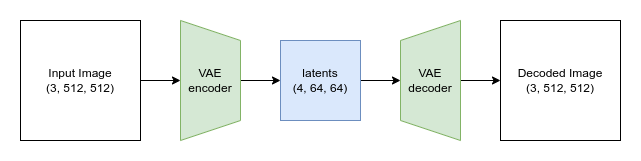
Figure 6. The VAE
Let’s load an image and see what it looks like after being compressed and decompressed by the VAE:
# NB, this will be our own image as part of the supplementary material to avoid external URLs
im = load_image('https://images.pexels.com/photos/14588602/pexels-photo-14588602.jpeg', size=(512, 512))
show_image(im);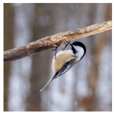
# Encode the image
with torch.no_grad():
    tensor_im = transforms.ToTensor()(im).unsqueeze(0).to(device)*2-1
    latent = vae.encode(tensor_im.half()) # Encode the image to a distribution
    latents = latent.latent_dist.sample() # Sampling from the distribution
    latents = latents * 0.18215 # This scaling factor was introduced by the SD authors to reduce the variance of the latents

latents.shape
torch.Size([1, 4, 64, 64])# Plot the individual channels of the latent representation
show_images([l for l in latents[0]], titles=[f'Channel {i}' for i in range(latents.shape[1])], ncols=4)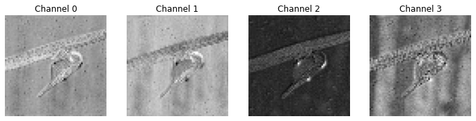
# Decode the image
with torch.no_grad():
    image = vae.decode(latents / 0.18215).sample
image = (image / 2 + 0.5).clamp(0, 1)
show_image(image[0].float());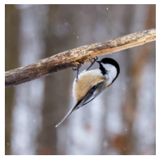
When generating images from scratch, we create a random set of latents as the starting point. We iteratively refine these noisy latents to generate a sample, and then the VAE decoder is used to deocde these final latents into an image we can view. The encoder is only used if we’d like to start the process from an existing image, something we’ll explore in chapter 6.
The UNet
The UNet used in stable diffusion is somewhat similar to the one we used in chapter 4 for generating images. Instead of taking in a 3-channel image as the input we take in a 4-channel latent. The timestep embedding is fed in the same way as the class conditioning was in the example at the start of this chapter. But this UNet also needs to accept the text embeddings as additional conditioning. Scattered throughout the UNet are cross-attention layers. Each spatial location in the UNet can ‘attend’ to different tokens in the text conditioning, bringing in relevant information from the prompt. The diagram in Figure 7 shows how this text conditioning (as well as timestep-based conditioning) is fed in at different points.

Figure 7. The Stable Diffusion UNet
The UNet for Stable Diffusion version 1 and 2 has around 860 million parameters. The more recent SD XL has even more, at around X billion, with most of the additional parameters being added at the lower-resolution stages via additional channels in the residual blocks (N vs 1280 in the original) and additional transformer blocks.
NB: This is speculation, the model has yet to be officially released so please don’t quote me on this ;)
Putting it All Together: Annotated Sampling Loop
Now that we know what each of the components does, let’s put them together to generate an image without relying on the pipeline. Here are the settings we’ll use:
# Some settings
prompt = ["Acrylic palette knife painting of a flower"] # What we want to generate
height = 512                        # default height of Stable Diffusion
width = 512                         # default width of Stable Diffusion
num_inference_steps = 30            # Number of denoising steps
guidance_scale = 7.5                # Scale for classifier-free guidance
seed = 42                           # Seed for random number generator
The first step is to encode the text prompt. Because we plan to do classifier-free guidance, we’ll actually create two sets of text embeddings: one with the prompt, and one representing an empty string. You can also encode a ‘negative prompt’ in place of the empty string, or combine multiple prompts with different weightings, but this is the most common usage:
# Tokenize the input
text_input = pipe.tokenizer(prompt, padding="max_length", max_length=pipe.tokenizer.model_max_length, truncation=True, return_tensors="pt")

# Feed through the text encoder
with torch.no_grad():
    text_embeddings = pipe.text_encoder(text_input.input_ids.to(device))[0]

# Do the same for the unconditional input (a blank string)
uncond_input = pipe.tokenizer("", padding="max_length", max_length=pipe.tokenizer.model_max_length, return_tensors="pt")
with torch.no_grad():
    uncond_embeddings = pipe.text_encoder(uncond_input.input_ids.to(device))[0]

# Concatenate the two sets of text embeddings embeddings
text_embeddings = torch.cat([uncond_embeddings, text_embeddings])
Next we create our random initial latents and set up the scheduler to use the desired number of inference steps:
# Prepare the Scheduler
pipe.scheduler.set_timesteps(num_inference_steps)

# Prepare the random starting latents
latents = torch.randn(
    (1, pipe.unet.in_channels, height // 8, width // 8), # Shape of the latent representation
    generator=torch.manual_seed(32),  # Seed the random number generator
).to(device).half()
latents = latents * pipe.scheduler.init_noise_sigma
Now we loop through the sampling steps, getting the model prediction at each stage and using this to update the latents:
# Sampling loop
for i, t in enumerate(pipe.scheduler.timesteps):

    # Create two copies of the latents to match the two text embeddings (unconditional and conditional)
    latent_model_input = torch.cat([latents] * 2)
    latent_model_input = pipe.scheduler.scale_model_input(latent_model_input, t)

    # predict the noise residual for both sets of inputs
    with torch.no_grad():
        noise_pred = pipe.unet(latent_model_input, t, encoder_hidden_states=text_embeddings).sample

    # Split the prediction into unconditional and conditional versions:
    noise_pred_uncond, noise_pred_text = noise_pred.chunk(2)

    # perform classifier-free guidance
    noise_pred = noise_pred_uncond + guidance_scale * (noise_pred_text - noise_pred_uncond)

    # compute the previous noisy sample x_t -> x_t-1
    latents = pipe.scheduler.step(noise_pred, t, latents).prev_sample
Notice the classifier-free guidance step. Our final noise prediction is noise_pred_uncond + guidance_scale * (noise_pred_text - noise_pred_uncond), pushing the prediction ‘away’ from the unconditional prediction towards the prediction made based on the prompt. Try changing the guidance scale to see how this affects the output.
By the end of the loop the latents should hopefully now represent a plausible image that matches the prompt. The final step is to decode the latents into an image using the VAE so that we can see the result:
# scale and decode the image latents with vae
latents = 1 / 0.18215 * latents
with torch.no_grad():
    image = vae.decode(latents).sample
image = (image / 2 + 0.5).clamp(0, 1)

# Display
show_image(image[0].float());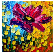
If you explore the source code for the StableDiffusionPipeline you’ll see that the code above closely matches the __call__ method used by the pipeline. Hopefully this annotated version shows that there is nothing too magical going on behind the scenes! Use this as a reference for when we encounter additional pipelines that add additional tricks to this foundation.
Open Data, Open Models
The LAION-5B dataset includes over 5 billion image-caption pairs scraped from the internet. This dataset was created by and for the open-source community, which saw the need for a publically-accessible dataset of this kind. Before the LAION initiative, only a handful of research labs at large companies had access to such data. These organizations kept the details of their private datasets to themselves, which made their results impossible to validate or replicate. By creating a publically available source of training data, LAION enabled a wave of smaller communities and organizations to train models and perform research that would otherwise have been impossible.
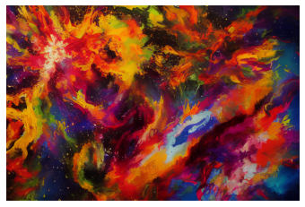
Figure 8: “An explosion of artistic creativity” - Image generated by the authors using Stable Diffusion
Stable Diffusion was one such model, trained on a subset of LAION as part of a collaboration between the researchers who had invented latent diffusion models and an organization called Stability AI. Training a model like SD requires a significant amount of GPU time. Even with the freely-available LAION dataset, there aren’t many who could afford the investment. This is why the public release of the model weights and code was such a big deal - it marked the first time a powerful text-to-image model with similar capabilities to the best closed-source alternatives was available to all. Stable Diffusion’s public availability has made it the go-to choice for researchers and developers looking to explore this technology over the past year. Hundreds of papers build upon the base model, adding new capabilities or finding innovative ways to improve its speed and quality. And innumerable startups have found ways to integrate these rapidly-improving tools into their products, spawning an entire ecosystem of new applications.
The months after the introduction of Stable Diffusion demonstrated the impact of sharing these technologies in the open. SD is not the best text-to-image model, but it IS the best model most of us had access to, so thousands of people have spent their time making it better and building upon that open foundation. We hope this example encourages others to follow suit and share their work with the open-source community in the future!
Summary
In this chapter we’ve seen how conditioning gives us new ways to control the images generated by diffusion models. We’ve seen how a text encoder can be used to condition a diffusion model on a text prompt, enabling powerful text-to-image capabilities. And we’ve explored how all of this comes together in the Stable Diffusion model by digging into the sampling loop and seeing how the different components work together. In the next chapter, we’ll show some of the many additional capabilities that can be added to diffusion models such as SD to take them beyond simple image generation. And later, in part 2 of the book, you’ll learn how to fine-tune SD to add new knowledge or capabilities to the model.