Diffusion Models

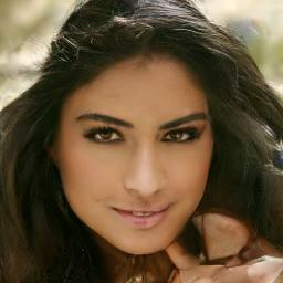
In late 2020 a little-known class of models called diffusion models began causing a stir in the machine-learning world. Researchers figured out how to use these diffusion models to generate higher-quality images than those produced by previous techniques. A flurry of papers followed, proposing improvements and modifications that pushed the quality up even further. By late 2021 there were models like GLIDE showcasing incredible results on text-to-image tasks, and a few months later, these models had entered the mainstream with tools like DALL-E 2 and Stable Diffusion. These models made it easy for anyone to generate images just by typing in a text description of what they wanted to see.

In this chapter, we’re going to dig into the details of how these models work. We’ll outline the key insights that make them so powerful, generate images with existing models to get a feel for how they work, and then train our own to deepen this understanding further. The field is still rapidly evolving, but the topics covered here should give you a solid foundation to build on, which will be extended further in chapters X, Y, and Z which take these ideas even further.

The Key Insight: Iterative Refinement

So what is it that makes diffusion models so powerful? Previous techniques, such as VAEs or GANs, generate their final output via a single forward pass of the model. This means the model must get everything right on the first try. If it makes a mistake, it can’t go back and fix it. Diffusion models, on the other hand, generate their output by iterating over many steps. This ‘iterative refinement’ allows the model to correct mistakes made in previous steps and gradually improve the output. To illustrate this, let’s look at an example of a diffusion model in action.

We can load a pre-trained model using the Hugging Face diffusers library. The pipeline can be used to create images directly, but this doesn’t show us what is going on under the hood:

# Load the pipeline
image_pipe = DDPMPipeline.from_pretrained("google/ddpm-celebahq-256")
image_pipe.to(device);

# Sample an image
image_pipe().images[0]

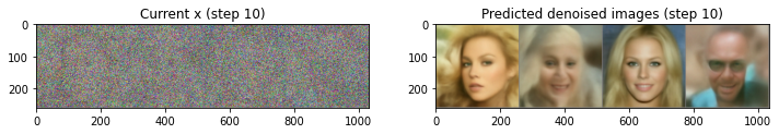
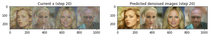
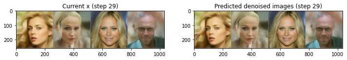
We can re-create the sampling process step by step to get a better look at what is happening under the hood. We initialize our sample x with random noise and then run it through the model for 30 steps. On the right, you can see the model’s prediction for what the final image will look like at specific steps - note that the initial predictions are not particularly good! Instead of jumping right to that final predicted image, we only modify x by a small amount in the direction of the prediction (shown on the left). We then feed this new, slightly better x through the model again for the next step, hopefully resulting in a slightly improved prediction, which can be used to update x a little more, and so on. With enough steps, the model can produce some impressively realistic images.

# The random starting point
x = torch.randn(4, 3, 256, 256).to(device)  # Batch of 4, 3-channel 256 x 256 px images

# Set the number of timesteps lower
image_pipe.scheduler.set_timesteps(num_inference_steps=30)

# Loop through the sampling timesteps
for i, t in enumerate(image_pipe.scheduler.timesteps):

    # Get the prediction given the current sample x and the timestep t
    with torch.no_grad():
        noise_pred = image_pipe.unet(x, t)["sample"]

    # Calculate what the updated sample should look like with the scheduler
    scheduler_output = image_pipe.scheduler.step(noise_pred, t, x)

    # Update x
    x = scheduler_output.prev_sample

    # Occasionally display both x and the predicted denoised images
    if i % 10 == 0 or i == len(image_pipe.scheduler.timesteps) - 1:
        fig, axs = plt.subplots(1, 2, figsize=(12, 5))

        grid = torchvision.utils.make_grid(x, nrow=4).permute(1, 2, 0)
        axs[0].imshow(grid.cpu().clip(-1, 1) * 0.5 + 0.5)
        axs[0].set_title(f"Current x (step {i})")

        pred_x0 = scheduler_output.pred_original_sample
        grid = torchvision.utils.make_grid(pred_x0, nrow=4).permute(1, 2, 0)
        axs[1].imshow(grid.cpu().clip(-1, 1) * 0.5 + 0.5)
        axs[1].set_title(f"Predicted denoised images (step {i})")
        plt.show()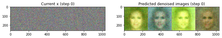

Note

Don’t worry if that chunk of code looks a bit intimidating - we’ll explain how this all works over the course of this chapter. For now, just focus on the results.

This core idea of learning how to refine a ‘corrupted’ input gradually can be applied to a wide range of tasks. In this chapter, we’ll focus on unconditional image generation, but diffusion models have also been applied to audio, video, text and more. And while most implementations use some variant of the ‘denoising’ approach that we’ll cover here, new approaches utilizing different types of ‘corruption’ together with iterative refinement are emerging that may move the field beyond the current focus on denoising diffusion specifically. Exciting times!

TODO: mention what unconditional means in the paragraph above

Training a Diffusion Model

In this section, we’re going to train a diffusion model from scratch to gain a better understanding of how they work. We’ll start by using components from the Hugging Face diffusers library. As the chapter progresses, we’ll gradually demystify how each component works. Training a diffusion model is relatively straightforward compared to other types of generative models. We repeatedly:

Load in some images from the training data.
Add noise in different amounts. Remember, we want the model to do a good job estimating how to ‘fix’ (denoise) both extremely noisy images and images that are close to perfect.
Feed the noisy versions of the inputs into the model.
Evaluate how well the model does at denoising these inputs.
Use this information to update the model weights.

To generate new images with a trained model, we begin with a completely random input and repeatedly feed it through the model, updating the input on each iteration by a small amount based on the model prediction. As we’ll see, there are a number of sampling methods that try to streamline this process so that we can generate good images with as few steps as possible.

The Data

For this example, we’ll use a dataset of images from the Hugging Face Hub- specifically, this collection of 1000 butterfly pictures. Later on, in the projects section, you will see how to use your own data.

dataset = load_dataset("huggan/smithsonian_butterflies_subset", split="train")

We need to do some preparation before this data can be used to train a model. Images are typically represented as a grid of ‘pixels’, with color values between 0 and 255 for each of the three color channels (Red, Green and Blue). To process these and make them ready for training, we: - Resize them to a fixed size - (Optional) Add some augmentation by randomly flipping them horizontally, effectively doubling the size of our dataset - Convert them to a PyTorch tensor (which represents the color values as floats between 0 and 1) - Normalize them to have a mean of 0, with values between -1 and 1

We can do all of this with torchvision.transforms:

image_size = 64

# Define data augmentations
preprocess = transforms.Compose(
    [
        transforms.Resize((image_size, image_size)),  # Resize
        transforms.RandomHorizontalFlip(),  # Randomly flip (data augmentation)
        transforms.ToTensor(),  # Convert to tensor (0, 1)
        transforms.Normalize([0.5], [0.5]),  # Map to (-1, 1)
    ]
)

Next, we need to create a dataloader to load the data in batches with these transforms applied:

batch_size = 32

def transform(examples):
    images = [preprocess(image.convert("RGB")) for image in examples["image"]]
    return {"images": images}


dataset.set_transform(transform)

train_dataloader = torch.utils.data.DataLoader(
    dataset, batch_size=batch_size, shuffle=True
)

We can check that this worked by loading a single batch and inspecting the images.

batch = next(iter(train_dataloader))
print('Shape:', batch['images'].shape, 
      '\nBounds:', batch['images'].min().item(), 'to', batch['images'].max().item())
show_images(batch['images'][:8]*0.5 + 0.5) # NB: we map back to (0, 1) for display

Shape: torch.Size([32, 3, 64, 64]) 
Bounds: -0.9921568632125854 to 1.0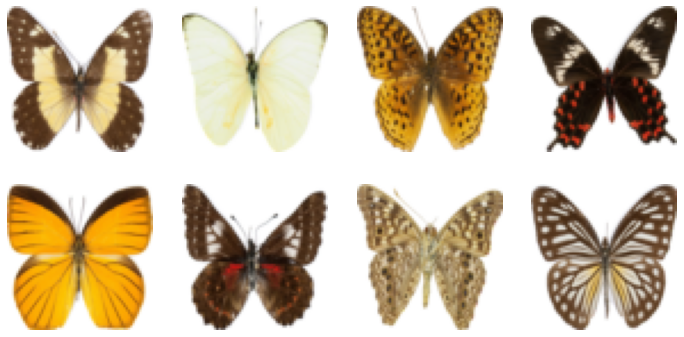

Adding Noise

How do we gradually corrupt our data? The most common approach is to add noise to the images. The amount of noise we add is controlled by a noise schedule. Different papers and approaches tackle this in different ways, which we’ll explore in section X. For now, let’s see one common approach in action based on the DDPM paper. In the diffusers library, adding noise is handled by something called a scheduler, which takes in a batch of images and a list of ‘timesteps’ and determines how to create the noisy versions of those images:

scheduler = DDPMScheduler(num_train_timesteps=1000, beta_start=0.001, beta_end=0.02)
timesteps = torch.linspace(0, 999, 8).long()

x = batch['images'][:8]
noise = torch.rand_like(x)
noised_x = scheduler.add_noise(x, noise, timesteps)
show_images((noised_x*0.5 + 0.5).clip(0, 1))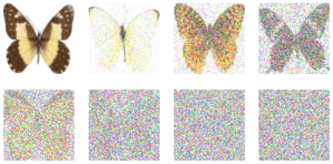

During training, we’ll pick the timesteps at random. The scheduler takes some parameters (beta_start and beta_end) which it uses to determine how much noise should be present for a given timestep. We will cover schedulers in more detail in section X.

The UNet

UNet is a convolutional neural network invented for tasks such as image segmentation, where the desired output has the same spatial extent as the input. It consists of a series of ‘downsampling’ layers that reduce the spatial size of the input, followed by a series of ‘upsampling’ layers that increase the spatial extent of the input again. The downsampling layers are also typically followed by a ‘skip connection’ that connects the downsampling layer’s output to the upsampling layer’s input. This allows the upsampling layers to ‘see’ the higher-resolution representations from earlier in the network, which is useful for tasks with image-like outputs where this high-resolution information is especially useful.

The UNet architecture used in the diffusers library is more advanced than the original UNet proposed in 2015 (TODO: add reference?), with additions like attention and residual blocks. We’ll take a closer look later, but the key feature here is that it can take in an input (the noisy image) and produce a prediction that is the same shape (the predicted noise). For diffusion models, the UNet typically also takes in the timestep as additional conditioning, which again we will explore in the UNet deep dive section. TODO reference somewhere.

Here’s how we might create a UNet and feed our batch of noisy images through it:

# Create a UNet2DModel
model = UNet2DModel(
    in_channels=3,  # 3 channels for RGB images
    sample_size=64,  # Specify our input size
    block_out_channels=(64, 128, 256, 512), # The number of channels per block affects the model size
    down_block_types=("DownBlock2D", "DownBlock2D", "AttnDownBlock2D", "AttnDownBlock2D"),
    up_block_types=("AttnUpBlock2D", "AttnUpBlock2D", "UpBlock2D", "UpBlock2D"),
)

# Pass a batch of data through
with torch.no_grad():
    out = model(noised_x, timestep=timesteps).sample
out.shape

torch.Size([8, 3, 64, 64])

Note that the output is the same shape as the input, which is exactly what we want.

Training

Now that we have our model and our data ready, we can train it. We’ll use the AdamW optimizer with a learning rate of 3e-4. For each training step, we: - Load a batch of images.

Add noise to the images, choosing random timesteps to determine how much noise is added.
Feed the noisy images into the model.
Calculate the loss, which is the mean squared error between the model’s predictions and the target - which in this case is the noise that we added to the images. This is called the noise or ‘epsilon’ objective. You can find more information on the different training objectives in section X.
Backpropagate the loss and update the model weights with the optimizer.

Here’s what all of that looks like in code:

num_epochs = 50 # How many runs through the data should we do?
lr = 1e-4 # What learning rate should we use
model = model.to(device) # The model we're training (defined in the previous section)
optimizer = torch.optim.AdamW(model.parameters(), lr=lr) # The optimizer
losses = [] # somewhere to store the loss values for later plotting

# Train the model (this takes a while!)
for epoch in range(num_epochs):
    for step, batch in enumerate(train_dataloader):
        
        # Load the input images
        clean_images = batch["images"].to(device)

        # Sample noise to add to the images
        noise = torch.randn(clean_images.shape).to(clean_images.device)

        # Sample a random timestep for each image
        timesteps = torch.randint(
            0,
            scheduler.num_train_timesteps,
            (clean_images.shape[0],),
            device=clean_images.device,
        ).long()

        # Add noise to the clean images according timestep
        noisy_images = scheduler.add_noise(clean_images, noise, timesteps)

        # Get the model prediction for the noise
        noise_pred = model(noisy_images, timesteps, return_dict=False)[0]

        # Compare the prediction with the actual noise:
        loss = F.mse_loss(noise_pred, noise)

        # Store the loss for later plotting
        losses.append(loss.item())

        # Update the model parameters with the optimizer based on this loss
        loss.backward(loss)
        optimizer.step()
        optimizer.zero_grad()

# Plot the loss curve:
plt.plot(losses);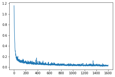

The loss curve trends downwards as the model learns to denoise the images. The curve is fairly noisy, thanks to different amounts of noise being added to the images based on the random sampling of timesteps for each iteration. It is hard to tell just by looking at the mean squared error of the noise predictions whether this model will be any good at generating samples, so let’s move on to the next section and see how well it does.

Sampling

The diffusers library uses the idea of ‘pipelines’ which bundle together all of the components needed to generate samples with a diffusion model:

pipeline = DDPMPipeline(unet=model, scheduler=scheduler)
ims = pipeline(batch_size=4).images
show_images(ims, nrows=1)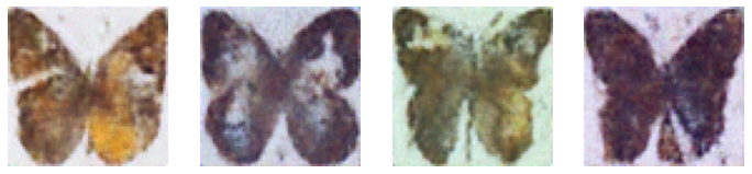

Of course, offloading the job of creating samples to the pipeline doesn’t really show us what is going on. So, here is a simple sampling loop that shows how the model is gradually refining the input image, based on the code contained in the pipeline’s __call__ method:

# Random starting point (4 random images):
sample = torch.randn(4, 3, 64, 64).to(device)

for i, t in enumerate(scheduler.timesteps):

    # Get model pred
    with torch.no_grad():
        noise_pred = model(sample, t).sample

    # Update sample with step
    sample = scheduler.step(noise_pred, t, sample).prev_sample

show_images(sample.clip(-1, 1)*0.5 + 0.5, nrows=1)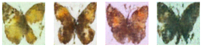

This is the same code we used at the beginning of the chapter to illustrate the idea of iterative refinement, but hopefully, now you have a better understanding of what is going on here. We start with a completely random input, which is then refined by the model in a series of steps. Each step is a small update to the input, based on the model’s prediction for the noise at that timestep. We’re still abstracting away some complexity behind the call to pipeline.scheduler.step() - in a later chapter we will dive deeper into different sampling methods and how they work.

Evaluation

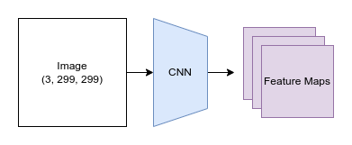
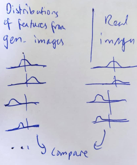
Generative model performance can be evaluated using FID scores (Fréchet Inception Distance). FID scores measure how closely generated samples match real-world samples by comparing statistics between feature maps extracted from both sets of data using a pre-trained neural network. The lower the score, the better the quality and realism of generated images produced by a given model. FID scores are popular due to their ability to provide an ‘objective’ comparison metric for different types of generative networks without relying on human judgment.

As convenient as FID scores are, there are some important caveats to be aware of: - The FID score for a given model depends on the number of samples used to calculate it, so when comparing between model,s we need to make sure both reported scores are calculated using the same number of samples. Common practice is to use 50,000 samples for this purpose, although to save time, you may evaluate on a smaller number of samples during development and only do the full evaluation once you’re ready to publish the results. - When calculating FID, images are resized to 299px square images. This makes it less useful as a metric for extremely low-res or high-res images. There are also minor differences between how resizing is handled by different deep learning frameworks, which can result in small differences in the FID score! We recommend using a library such as clean-fid to standardize the FID calculation. - The network used as a feature extractor for FID is typically a model trained on the Imagenet classification task. When generating images in a different domain, the features learned by this model may be less useful. A more accurate approach would be to somehow train a classification network on domain-specific data first, but this would make it harder to compare scores between different papers and approaches, so for now the imagenet model is the standard choice. - If you save generated samples for later evaluation, the format and compression can again affect the FID score. Avoid low-quality JPEG images where possible.

Even if you account for all these caveats, FID scores are just a rough measure of quality and do not perfectly capture the nuances of what makes images look more ‘real’. So, use them to get an idea of how one model performs relative to another but also look at the actual images generated by each model to get a better sense of how they compare. Human preference is still the gold standard for quality in what is ultimately a fairly subjective field!

In Depth: Noise Schedules

In the training example above, one of the steps was ‘add noise, in different amounts’. We achieved this by picking a random timestep between 0 and 1000 and then relying on the scheduler to add the appropriate amount of noise. Likewise, during sampling, we again relied on the scheduler to tell us which timesteps to use and how to move from one to the next given the model predictions. It turns out that choosing how much noise to add is an important design decision that can drastically affect the performance of a given model. In this section, we’ll see why this is the case and explore some of the different approaches that are used in practice.

Why Add Noise?

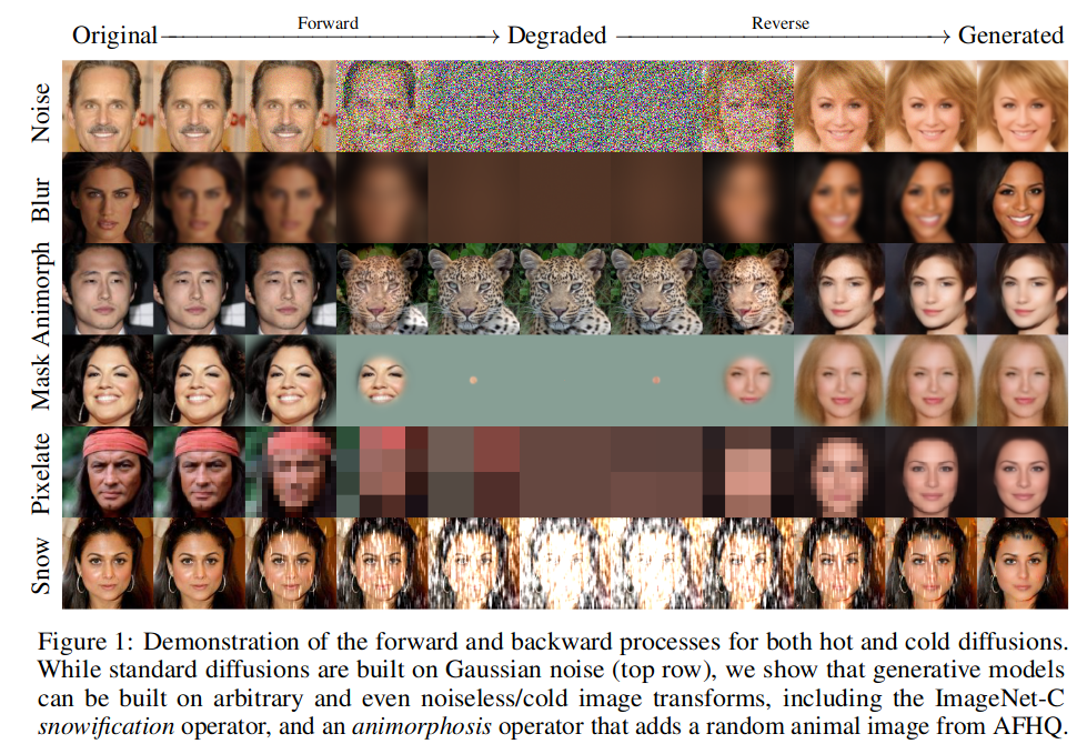
[image from cold diffusion paper]

At the start of this chapter, we said that the key idea behind diffusion models is that of iterative refinement. During training, we ‘corrupt’ an input by different amounts. During inference, we begin with a ‘maximally corrupted’ input and iteratively ‘de-corrupt’ it, in the hopes that we will eventually end up with a nice final result.

So far, we’ve focused on one specific kind of ‘corruption’: adding Gaussian noise. One reason for this is the theoretical underpinnings of diffusion models - if we use a different corruption method we are no longer technically doing ‘diffusion’! However, a paper titled ‘Cold Diffusion’ [TODO ref] dramatically demonstrated that we do not necessarily need to constrain ourselves to this method just for theoretical convenience. They showed that a diffusion-model-like approach works for many different ‘corruption’ methods (see figure TODO). More recently, [MUSE]/[MaskGIT]/[PAELLA] have used random token masking or replacement as an equivalent ‘corruption’ method for quantized data - that is, data that is represented by discrete tokens rather than continuous values.

Nonetheless, adding noise remains the most popular approach for several reasons: - We can easily control the amount of noise added, giving a smooth transition from ‘perfect’ to ‘completely corrupted’. This is not the case for something like reducing the resolution of an image, which may result in ‘discrete’ transitions. - We can have many valid random starting points for inference, unlike some methods which may only have a limited number of possible initial (fully corrupted) states, such as a completely black image or a single-pixel image.

So, for the moment at least, we’ll stick with adding noise as our corruption method. Next, let’s take a closer look at how we add noise to our images.

Starting Simple

We have some images (x) and we’d like to combine them somehow with some random noise.

x = next(iter(train_dataloader))['images'][:8]
noise = torch.rand_like(x)

One way we could do this is to linearly interpolate (lerp) between them by some amount. This gives us a function that smoothly transitions from the original image x to pure noise as the ‘amount’ varies from 0 to 1:

def corrupt(x, noise, amount):
  amount = amount.view(-1, 1, 1, 1) # make sure it's broadcastable
  return x*(1-amount) + noise*amount # equivalent to x.lerp(noise, amount) TODO maybe replace with this?

Let’s see this in action on a batch of data, with the amount of noise varying from 0 to 1:

amount = torch.linspace(0, 1, 8)
noised_x = corrupt(x, noise, amount)
show_images(noised_x*0.5 + 0.5)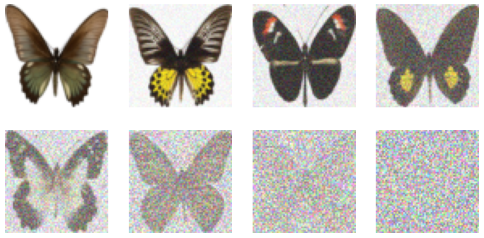

This seems to be doing exactly what we want, smoothly transitioning from the original image to pure noise. Now, we’ve created a noise schedule here that takes in a value for ‘amount’ from 0 to 1. This is called the ‘continuous time’ approach, where we represent the full path on a time scale from 0 to 1. Other approaches use a discrete time approach, with some large integer number of ‘timesteps’ used to define the noise scheduler. We can wrap our function into a class that converts from continuous time to discrete timesteps and adds noise appropriately:

class SimpleScheduler():
  def __init__(self):
    self.num_train_timesteps = 1000
  def add_noise(self, x, noise, timesteps):
    amount = timesteps / self.num_train_timesteps
    return corrupt(x, noise, amount)

scheduler = SimpleScheduler()
timesteps = torch.linspace(0, 999, 8).long()
noised_x = scheduler.add_noise(x, noise, timesteps)
show_images(noised_x*0.5 + 0.5)

Now we have something that we can directly compare to the schedulers used in the diffusers library, such as the DDPMScheduler we used during training. Let’s see how it compares:

scheduler = DDPMScheduler(beta_end=0.01)
timesteps = torch.linspace(0, 999, 8).long()
noised_x = scheduler.add_noise(x, noise, timesteps)
show_images((noised_x*0.5 + 0.5).clip(0, 1))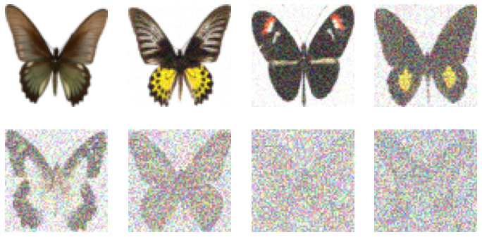

The Maths

There are many competing notations and approaches in the literature. For example, some papers parametrize the noise schedule in ‘continuous-time’ where t runs from 0 (no noise) to 1 (fully corrupted) - just like our corrupt function in the previous section. Others use a ‘discrete-time’ approach with integer timesteps running from 0 to some large number T, typically 1000. It is possible to convert between these two approaches the way we did with our ‘SimpleScheduler’ class - just make sure you’re consistent when comparing different models. We’ll stick with the discrete-time approach here.

A good place to start for pushing deeper into the maths is the paper DDPM TODO ref. You can find an annotated implementation https://huggingface.co/blog/annotated-diffusion which is a great additional resource. TODO reference better.

The paper begins by specifying a single noise step to go from timestep t-1 to timestep t. Here’s how they write it:

\[ q(\mathbf{x}_t | \mathbf{x}_{t-1}) = \mathcal{N}(\mathbf{x}_t; \sqrt{1 - \beta_t} \mathbf{x}_{t-1}, \beta_t \mathbf{I}). \]

Here $\beta_t$ is defined for all timesteps t and is used to specify how much noise is added at each step. This notation can be a little intimidating, but what this equation tells us is that the noisier $\mathbf{x}_t$ is a distribution with a mean of $\sqrt{1 - \beta_t} \mathbf{x}_{t-1}$ and a variance of $\beta_t$. In other words, $\mathbf{x}_t$ is a mix of $\mathbf{x}_{t-1}$ (scaled by $\sqrt{1 - \beta_t}$) and some random noise, which we can think of as unit-variance noise scaled by $\sqrt{\beta_t}$. Given $x_{t-1}$ and some noise $\epsilon$, we can sample from this distribution to get $x_t$ with:

\[ \mathbf{x}_t = \sqrt{1 - \beta_t} \mathbf{x}_{t-1} + \sqrt{\beta_t} \mathbf{\epsilon} \]

To get the noisy input at timestep t, we could begin at t=0 and repeatedly apply this single step, but this would be very inefficient. Instead, we can find a formula to move to any timestep t in one go. We define $\alpha_t = 1 - \beta_t$ and then use the following formula:

\[ x_t = \sqrt{\bar{\alpha}_t}x_0 + \sqrt{1-\bar{\alpha}_t}\epsilon \]

where - $\epsilon$ is some gaussian noise with unit variance - $\bar{\alpha}$ (‘alpha_bar’) is the cumulative product of all the $\alpha$ values up to the time $t$.

So $x_t$ is a mixture of $x_0$ (scaled by $\sqrt{\bar{\alpha}_t}$) and $\epsilon$ (scaled by $\sqrt{1-\bar{\alpha}_t}$). In the diffusers library the $\bar{\alpha}$ values are stored in scheduler.alphas_cumprod. Knowing this, we can plot the scaling factors for the original image $x_0$ and the noise $\epsilon$ across the different timesteps for a given scheduler:

plot_scheduler(DDPMScheduler(beta_start=0.001, beta_end=0.02, beta_schedule="linear")) # The default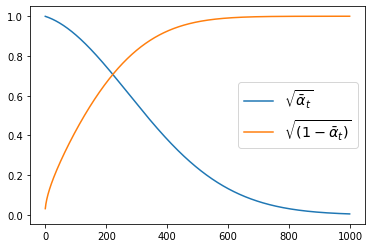

Our SimpleScheduler above just linearly mixes between the original image and noise, as we can see if we plot the scaling factors (equivalent to ${\sqrt{\bar{\alpha}_t}}$ and $\sqrt{(1 - \bar{\alpha}_t)}$ in the DDPM case):

plot_scheduler(SimpleScheduler())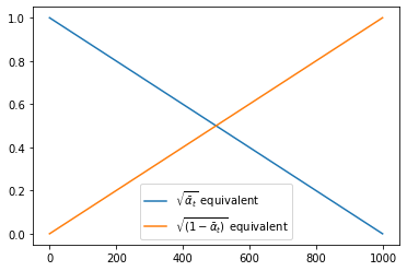

A good noise schedule will ensure that the model sees a mix of images at different noise levels. The best choice will differ based on the training data. Visualizing a few more options, note that: - Setting beta_end too low means we never completely erase the image, so the model will never see anything like the random noise used as a starting point for inference. - Setting beta_end extremely high means that most of the timesteps are spent on almost complete noise, which will result in poor training performance. - Different beta schedules give different curves. The ‘cosine’ schedule is a popular choice, as it gives a smooth transition from the original image to the noise.

fig, (ax) = plt.subplots(1, 1, figsize=(8, 5))
plot_scheduler(DDPMScheduler(beta_schedule="linear"), label = 'default schedule', ax=ax, plot_both=False)
plot_scheduler(DDPMScheduler(beta_schedule="squaredcos_cap_v2"), label = 'cosine schedule', ax=ax, plot_both=False)
plot_scheduler(DDPMScheduler(beta_start=0.001, beta_end=0.003, beta_schedule="linear"), label = 'Low beta_end', ax=ax, plot_both=False)
plot_scheduler(DDPMScheduler(beta_start=0.001, beta_end=0.1, beta_schedule="linear"), label = 'High beta_end', ax=ax, plot_both=False)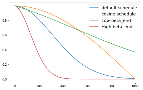

Note

All of the schedules shown here are called ‘Variance Preserving’ (VP), meaning that the variance of the model input is kept close to 1 across the entire schedule. You may also encounter ‘Variance Exploding’ (VE) formulations where noise is simply added to the original image in different amounts (resulting in high-variance inputs). We’ll go into this more in the chapter on sampling. Our SimpleScheduler is almost a VP schedule, but the variance is not quite preserved due to the linear interpolation.

As with many diffusion-related topics, there is a constant stream of new papers exploring the topic of noise schedules, so by the time you read this there will likely be a large collection of options to try out!

Effect of Input Resolution and Scaling

One aspect of noise schedules that was mostly overlooked until recently is the effect of input size and scaling. Many papers test potential schedulers on small-scale datasets and at low resolution, and then use the best-performing scheduler to train their final models on larger images. The problem with this is can be seen if we add the same amount of noise to two images of different sizes:

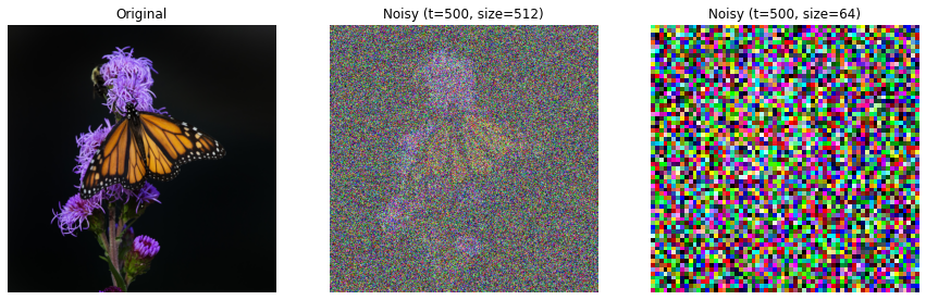
Images at high resolution tend to contain a lot of redundant information. This means that even if a single pixel is obscured by noise, the surrounding pixels contain enough information to reconstruct the original image. This is not the case for low-resolution images, where a single pixel can contain a lot of information. This means that adding the same amount of noise to a low-resolution image will result in a much more corrupted image than adding the equivalent amount of noise to a high-resolution image.

This effect was thoroughly investigated in two independent papers, both of which came out in January 2023. Each used the new insights to train models capable of generating high-resolution outputs without requiring any of the tricks that have previously been necessary. [simple diffusion] introduced a method for adjusting the noise schedule based on the input size, allowing a schedule optimized on low-resolution images to be appropriately modified for a new target resolution. [Cheng] performed similar experiments, and noted another key variable: input scaling. That is, how do we represent our images? If the images are represented as floats between 0 and 1 then they will have a lower variance than the noise (which is typically unit variance) and thus the signal-to-noise ratio will be lower for a given noise level than if the images were represented as floats between -1 and 1 (which we used in the training example above) or something else. Scaling the input images shifts the signal-to-noise ratio, and so modifying this scaling is another way we can adjust when training on larger images.

In Depth: UNets and Alternatives

Now let’s address the actual model that makes the all-important predictions! To recap, this model must be capable of taking in a noisy image and estimating how to denoise it. This requires a model that can take in an image of arbitrary size and output an image of the same size. Furthermore, the model should be able to make precise predictions at the pixel level, while also capturing higher-level information about the image as a whole. A popular approach is to use an architecture called a UNet. UNets were invented in 2015 (TODO check date) for medical image segmentation, and have since become a popular choice for various image-related tasks. Like the AutoEncoders and VAEs we looked at in the previous chapter, UNets are made up of a series of ‘downsampling’ and ‘upsampling’ blocks. The downsampling blocks are responsible for reducing the size of the image, while the upsampling blocks are responsible for increasing the size of the image. The downsampling blocks are typically made up of a series of convolutional layers, followed by a pooling or downsampling layer. The upsampling blocks are typically made up of a series of convolutional layers, followed by an upsampling or ‘transposed convolution’ layer. The transposed convolution layer is a special type of convolutional layer that increases the size of the image, rather than reducing it.

The reason a regular AutoEncoder or VAE is not a good choice for this task is that they are less capable of making precise predictions at the pixel level since the output must be entirely re-constructed from the low-dimensional latent space. In a UNet, the downsampling and upsampling blocks are connected by ‘skip connections’, which allow information to flow directly from the downsampling blocks to the upsampling blocks. This allows the model to make precise predictions at the pixel level, while also capturing higher-level information about the image as a whole.

A Simple UNet

To better understand the structure of a UNet, let’s build a simple UNet from scratch.

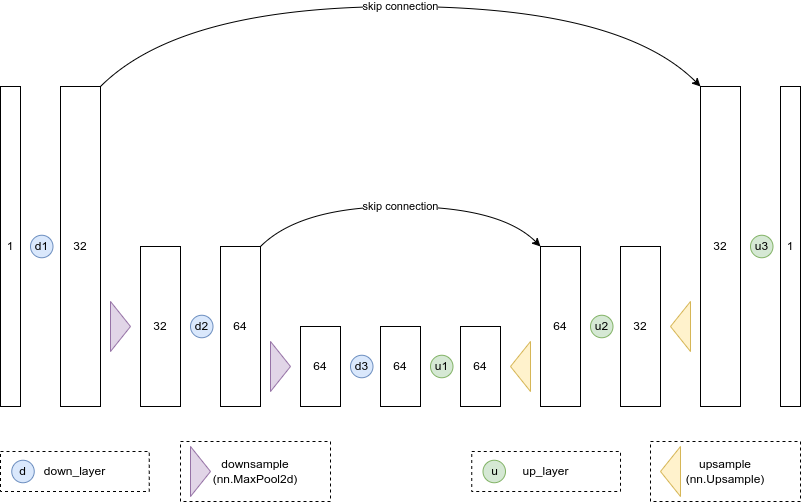
This UNet takes single-channel inputs at 32px resolution and outputs single-channel outputs at 32px resolution, which we could use to build a diffusion model for the MNIST dataset. There are three layers in the encoding path, and three layers in the decoding path. Each layer consists of a convolution followed by an activation function and an upsampling or downsampling step (depending on whether we are in the encoding or decoding path). The skip connections allow information to flow directly from the downsampling blocks to the upsampling blocks, and are implemented by adding the output of the downsampling block to the input of the corresponding upsampling block. Some UNets instead concatenate the output of the downsampling block to the input of the corresponding upsampling block, and may also include additional layers in the skip connections. Here’s what this network looks like in code:

from torch import nn

class BasicUNet(nn.Module):
    """A minimal UNet implementation."""
    def __init__(self, in_channels=1, out_channels=1):
        super().__init__()
        self.down_layers = torch.nn.ModuleList([ 
            nn.Conv2d(in_channels, 32, kernel_size=5, padding=2),
            nn.Conv2d(32, 64, kernel_size=5, padding=2),
            nn.Conv2d(64, 64, kernel_size=5, padding=2),
        ])
        self.up_layers = torch.nn.ModuleList([
            nn.Conv2d(64, 64, kernel_size=5, padding=2),
            nn.Conv2d(64, 32, kernel_size=5, padding=2),
            nn.Conv2d(32, out_channels, kernel_size=5, padding=2), 
        ])
        self.act = nn.SiLU() # The activation function
        self.downscale = nn.MaxPool2d(2)
        self.upscale = nn.Upsample(scale_factor=2)

    def forward(self, x):
        h = []
        for i, l in enumerate(self.down_layers):
            x = self.act(l(x)) # Through the layer and the activation function
            if i < 2: # For all but the third (final) down layer:
              h.append(x) # Storing output for skip connection
              x = self.downscale(x) # Downscale ready for the next layer
              
        for i, l in enumerate(self.up_layers):
            if i > 0: # For all except the first up layer
              x = self.upscale(x) # Upscale
              x += h.pop() # Fetching stored output (skip connection)
            x = self.act(l(x)) # Through the layer and the activation function
            
        return x

A diffusion model trained with this architecture on MNIST produces the following samples (code included in the supplementary material but omitted here for brevity):

Improving the UNet

This simple UNet works for this relatively easy task, but it is far from ideal. So, what can we do to improve it? - Add more parameters. This can be accomplished by using multiple convolutional layers in each block, by using a larger number of filters in each convolutional layer, or by making the network deeper. - Add residual connections. Using ResBlocks instead of regular convolutional layers can help the model learn more complex functions while keeping training stable. - Add normalization, such as batch normalization. Batch normalization can help the model learn more quickly and reliably, by ensuring that the outputs of each layer are centered around 0 and have a standard deviation of 1. - Add regularization, such as dropout. Dropout helps by preventing the model from overfitting to the training data, which is important when working with smaller datasets. - Add attention. By introducing self-attention layers we allow the model to focus on different parts of the image at different times, which can help it learn more complex functions. The addition of transformer-like attention layers also lets us increase the number of learnable parameters, which can help the model learn more complex functions. The downside is that attention layers are much more expensive to compute than regular convolutional layers at higher resolutions, so we typically only use them at lower resolutions (i.e. the lower resolution blocks in the UNet).

For comparison, here are the results on MNIST when using the UNet implementation in the diffusers library, which features all of the above improvements:

Caution

This section will likely be expanded with results and more details in the future. We just haven’t gotten around to training variants with the different improvements yet!

Alternative Architectures

Diagram: Comparing UNet with UVit and RIN (TODO)

More recently, a number of alternative architectures have been proposed for diffusion models. These include: - Transformers. The [DIT PAPER TODO LINK] showed that a transformer-based architecture can be used to train a diffusion model, with great results. However, the compute and memory requirements of the transformer architecture remain a challenge for very high resolutions. - The ‘UViT’ architecture from the ‘Simple Diffusion’ paper TODO link aims to get the best of both worlds by replacing the middle layers of the UNet with a large stack of transformer blocks. A key insight of this paper was that focusing the majority of the compute at the lower resolution blocks of the UNet allows for more efficient training of high-resolution diffusion models. For very high resolutions, they do some additional pre-processing using something called a wavelet transform to reduce the spatial resolution of the input image while keeping as much information as possible through the use of additional channels, again reducing the amount of compute spent on the higher spatial resolutions. - Recurrent Interface Networks. The [RIN PAPER TODO LINK] takes a similar approach, first mapping the high-resolution inputs to a more manageable and lower-dimensional ‘latent’ representation which is then processed by a stack of transformer blocks before being decoded back out to an image. Additionally, the RIN paper introduces an idea of ‘recurrence’ where information is passed to the model from the previous processing step, which can be beneficial for the kind of iterative improvement that diffusion models are designed to perform.

It remains to be seen whether transformer-based approaches completely supplant UNets as the go-to architecture for diffusion models, or whether hybrid approaches like the UViT and RIN architectures will prove to be the most effective.

In Depth: Objectives and Pre-Conditioning (TODO)

We’ve spoken about diffusion models taking a noisy input and “learning to denoise” it. At first glance, you might assume that the natural prediction target for the network is the denoised version of the image, which we’ll call x0. However, in the code, we compared the model prediction with the unit-variance noise that was used to create the noisy version (often called the epsilon objective, eps). The two appear mathematically identical since if we know the noise and the timestep we can derive x0 and vice versa. While this is true, the choice of objective has some subtle effects on how large the loss is at different timesteps, and thus which noise levels the model learns to denoise best. To gain some intuition, let’s visualize some different objectives across different timesteps:

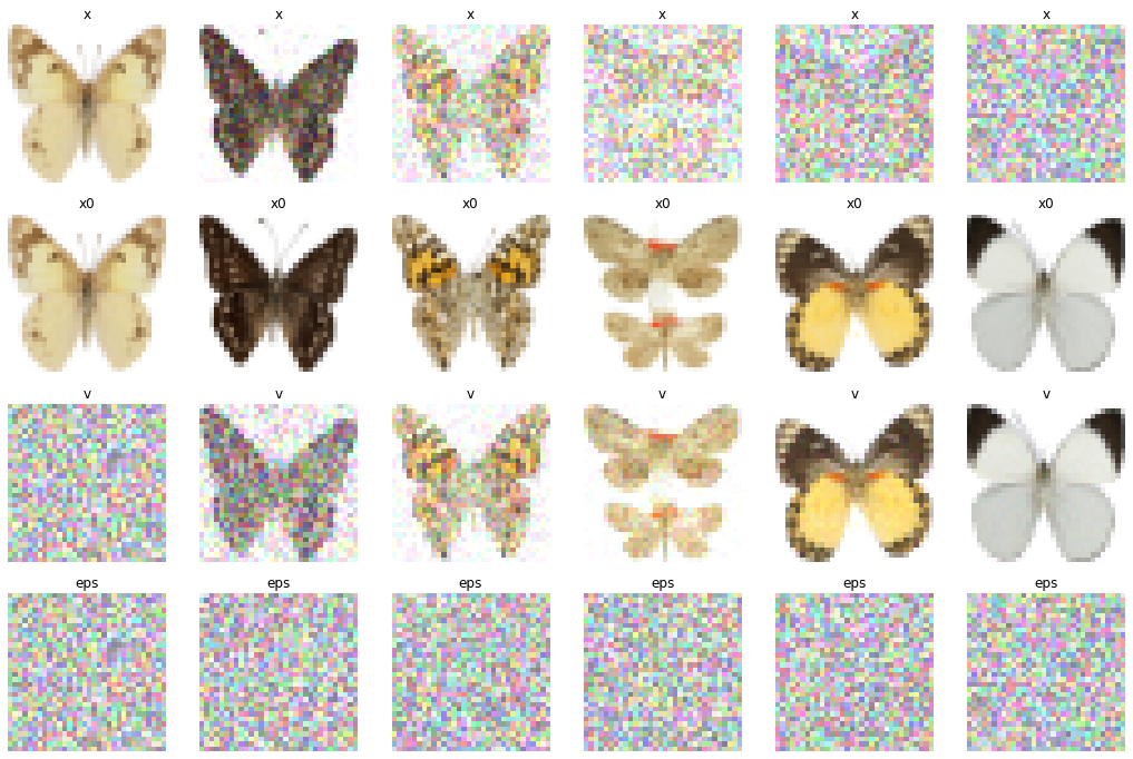
At extremely low noise levels, the x0 objective is trivially easy while predicting the noise accurately is almost impossible. Likewise, at extremely high noise levels, the eps objective is easy while predicting the denoised image accurately is almost impossible. Neither case is ideal, and so additional objectives have been introduced that have the model predict a mix of x0 and eps at different timesteps. The v objective is one such objective, which is defined as $ v = + x_0 $. Karras et al (TODO cite properly) introduce a similar idea via a parameter called c_skip, and unify the different diffusion model formulations into a consistent framework. If you’re interested in learning more about the different objectives, scalings and other nuances of the different diffusion model formulations, we recommend reading [EDM] for a more in-depth discussion.

Project Time: Train Your Own Diffusion Model (TODO)

“OK that’s enough theory go try it yourself” (TODO) Ref supplementary materials where we can put nice code for dealing with different data formats etc Doesn’t need to have too much detail.

Summary (TODO)

Needs a nice summary and probably a further reading section (Karras, Salimans, Cheng, Diffusion Models, DDPM, etc.)