CCLDDG Core Class

Defining the key UNet and Discriminator architectures used.

Building Blocks

This section defines the different building blocks we’ll use to build the core unet and discriminator architectures.

The activation function:

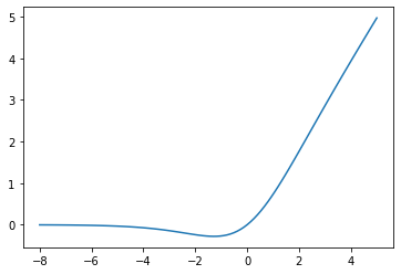
By default this all uses the Swish activation function: \(x \cdot \sigma(x)\)

---

source

Swish

 Swish ()

swish…

You can think of this as ‘fancy ReLU’… This is what it looks like:

Code

swish = Swish()
x = torch.linspace(-8, 5, 100)
y = swish(x)
plt.plot(x, y)
plt.show()

Embeddings

Next, we want a way to create embeddings from various conditioning information.

---

source

TimeEmbedding

 TimeEmbedding (n_channels:int, denom_factor=10000)

Embeddings for \(t\)

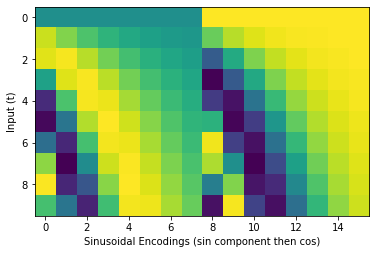
The Positional Embedding used for TimeEmbedding is a sinusoidal embedding as used in many transformer implementations: \[ \begin{align} PE^{(1)}_{t,i} &= sin\Bigg(\frac{t}{10000^{\frac{i}{d - 1}}}\Bigg) \\ PE^{(2)}_{t,i} &= cos\Bigg(\frac{t}{10000^{\frac{i}{d - 1}}}\Bigg) \end{align} \]

where \(d\) is half_dim = n_channels//8

Since we expect to encode only a small number of steps we can specify a smaller multiplier than 10000 using the denom_factor argument.

These sinusoidal embeddings are usually then passed through an MLP to transform them into n_channels outputs, but we can pass in return_sinusoidal_embs=True to get the raw sinusoidal embeddings for visualization purposes. Here’s an example visualizing this for t in range(0, 10):

Code

te = TimeEmbedding(n_channels=64, denom_factor=16)
t = torch.arange(0, 10)
embs = te(t, return_sinusoidal_embs=True)
embs.shape
plt.imshow(embs.detach(), )
plt.xlabel('Sinusoidal Encodings (sin component then cos)')
plt.ylabel('Input (t)')
plt.show()

We also create embeddings to map a latent variable z and our CLOOB embedding to set numbers of channels. Both simply run the input through a small MLP to map them to n_channels outputs.

---

source

ZEmbedding

 ZEmbedding (z_dim:int, n_channels:int)

Embedding to map a latent z (z_dim dimensions) to n_channels via an MLP

---

source

CLOOBEmbedding

 CLOOBEmbedding (n_channels:int)

Embedding to map a CLOOB embedding (512 dimensions) to n_channels via an MLP

Additional Components

The rest of the building blocks are fairly standard, but all here take both an input (x) and some conditioning (cond).

---

source

Downsample

 Downsample (n_channels)

Scale down the feature map by 0.5

---

source

Upsample

 Upsample (n_channels)

Scale up the feature map by 2.

---

source

MiddleBlock

 MiddleBlock (n_channels:int, n_cond_channels:int)

Middle block

It combines a ResidualBlock, AttentionBlock, followed by another ResidualBlock. This block is applied at the lowest resolution of the U-Net.

---

source

UpBlock

 UpBlock (in_channels:int, out_channels:int, n_cond_channels:int,
          has_attn:bool)

Up block

This combines ResidualBlock and AttentionBlock. These are used in the second half of U-Net at each resolution.

---

source

DownBlock

 DownBlock (in_channels:int, out_channels:int, time_channels:int,
            has_attn:bool)

Down block

This combines ResidualBlock and AttentionBlock. These are used in the first half of U-Net at each resolution.

---

source

AttentionBlock

 AttentionBlock (n_channels:int, n_heads:int=1, d_k:int=None,
                 n_groups:int=32)

Attention block

This is similar to transformer multi-head attention.

---

source

ResidualBlock

 ResidualBlock (in_channels:int, out_channels:int, n_cond_channels:int,
                n_groups:int=32)

Residual block

A residual block has two convolution layers with group normalization. Each resolution is processed with two residual blocks.

The UNet and Discriminator

This is what we’ve been building up to. We want a UNet mode that can take in a (noisy) image or image-like tensor, along with some conditioning information (timestep, CLOOB embedding) and optionally a latent z, and produce an output of the same shape as the input.

---

source

UNet

 UNet (image_channels:int=3, n_channels:int=64,
       ch_mults:Union[Tuple[int,...],List[int]]=(1, 2, 2, 4),
       is_attn:Union[Tuple[bool,...],List[int]]=(False, False, True,
       True), n_blocks:int=2, use_z=True, z_dim:int=8,
       n_z_channels:int=16, use_cloob=True, n_cloob_channels:int=256,
       n_time_channels:int=-1, denom_factor:int=100)

U-Net

Hopefully flexible enough :) Arguments:

* `image_channels` is the number of channels in the image. $3$ for RGB.
* `n_channels` is number of channels in the initial feature map that we transform the image into
* `ch_mults` is the list of channel numbers at each resolution. The number of channels is `ch_mults[i] * n_channels`
* `is_attn` is a list of booleans that indicate whether to use attention at each resolution
* `n_blocks` is the number of `UpDownBlocks` at each resolution
* `use_z`=True. Set to false if you don't want to include the latent z input
* `z_dim` is the dimension of the latent `z`, and `n_z_channels` is the size of the embedding used for it.
* `use_cloob` = True. Set to false if you don't want to use CLOOB conditioning.
* `n_cloob_channels` - the size of the embedding used for the CLOOB conditioning input.
* `n_time_channels` - the size of the time embedding. If -1, this is set to n_channels*4
* `denom_factor` for the TimeEmbedding. 100 by default, set to 10,000 if wanting to do more traditional diffusion stuff where n_steps is high.

We’d also like a Discriminator that can take in an image, with the same optional conditioning information, and spit out a classification (real or fake). If you want to condition the discriminator on another image (e.g. in DDG the discriminator takes in \(x_{t-1}\) and is conditioned on \(x_t\)) then simply concatenate them together and use image_channels = 2*[the number of channels in a single image].

---

source

Discriminator

 Discriminator (image_channels:int=3, n_channels:int=64,
                ch_mults:Union[Tuple[int,...],List[int]]=(1, 2, 2, 4),
                is_attn:Union[Tuple[bool,...],List[int]]=(False, False,
                True, True), n_blocks:int=2, use_cloob=True,
                n_cloob_channels:int=256, n_time_channels:int=-1,
                denom_factor:int=100)

Discriminator

Based on the same architecture as the UNet, but without the upwards half. Arguments:

* `image_channels` is the number of channels in the image. $3$ for RGB.
* `n_channels` is number of channels in the initial feature map that we transform the image into
* `ch_mults` is the list of channel numbers at each resolution. The number of channels is `ch_mults[i] * n_channels`
* `is_attn` is a list of booleans that indicate whether to use attention at each resolution
* `n_blocks` is the number of `UpDownBlocks` at each resolution
* `use_cloob` = True. Set to false if you don't want to use CLOOB conditioning.
* `n_cloob_channels` - the size of the embedding used for the CLOOB conditioning input.
* `n_time_channels` - the size of the time embedding. If -1, this is set to n_channels*4
* `denom_factor` for the TimeEmbedding. 100 by default, set to 10,000 if wanting to do more traditional diffusion stuff where n_steps is high.

Let’s see both in action:

device = 'cpu'
unet = UNet(image_channels=4).to(device)
z = torch.randn((1,8), device=device)
c = torch.zeros((1,512), device=device)
x = torch.randn(1, 4, 16, 16).to(device)
t = torch.tensor(3, dtype=torch.long).unsqueeze(0).to(device)
pred_im = unet(x.float(), t, c, z)
x.shape, pred_im.shape

(torch.Size([1, 4, 16, 16]), torch.Size([1, 4, 16, 16]))

disc = Discriminator(image_channels=4, use_cloob=False)
disc(x, t).shape

torch.Size([1, 1])

labels = torch.tensor([1]).float()
criterion = nn.BCELoss()
criterion(disc(x, t).view(-1), labels)

tensor(0.6967, grad_fn=<BinaryCrossEntropyBackward0>)